The Biodiversity Crisis
By the end of this section, you will be able to:
- Define biodiversity in terms of species diversity and abundance
- Describe biodiversity as the equilibrium of naturally fluctuating rates of extinction and speciation
- Identify historical causes of high extinction rates in Earth’s history
Traditionally, ecologists have measured biodiversity, a general term for the number of species present in the biosphere, by taking into account both the number of species and their relative abundance to each other. Biodiversity can be estimated at a number of levels of organization of living organisms. These estimation indices, which came from information theory, are most useful as a first step in quantifying biodiversity between and within ecosystems; they are less useful when the main concern among conservation biologists is simply the loss of biodiversity. However, biologists recognize that measures of biodiversity, in terms of species diversity, may help focus efforts to preserve the biologically or technologically important elements of biodiversity.
The Lake Victoria cichlids provide an example with which we can begin to understand biodiversity. The biologists studying cichlids in the 1980s discovered hundreds of cichlid species representing a variety of specializations to specialized habitat types and specific feeding strategies: such as eating plankton floating in the water, scraping/eating algae from rocks, eating insect larvae from the lake bottom, and eating the eggs of other species of cichlid. The cichlids of Lake Victoria are the product of a complex adaptive radiation. An adaptive radiation is a rapid (less than three million years in the case of the Lake Victoria cichlids) branching through speciation of a phylogenetic clade into many closely related species. Typically, the species “radiate” into different habitats and niches. The Galápagos Island finches are an example of a modest adaptive radiation with 15 species. The cichlids of Lake Victoria are an example of a spectacular adaptive radiation that formerly included about 500 species.
At the time biologists were making this discovery, some species began to quickly disappear. A culprit in these declines was the Nile perch, a species of large predatory fish that was introduced to Lake Victoria by fisheries to feed the people living around the lake. The Nile perch was introduced in 1963, but its populations did not begin to surge until the 1980s. The perch population grew by consuming cichlids, driving species after species to the point of extinction (the disappearance of a species). In fact, there were several factors that played a role in the extinction of perhaps 200 cichlid species in Lake Victoria: the Nile perch, declining lake water quality due to agriculture and land clearing on the shores of Lake Victoria, and increased fishing pressure. Scientists had not even catalogued all of the species present—so many were lost that were never named. The diversity is now a shadow of what it once was.
The cichlids of Lake Victoria are a thumbnail sketch of contemporary rapid species loss that occurs all over Earth that is caused primarily by human activity. Extinction is a natural process of macroevolution that occurs at the rate of about one out of 1 million species becoming extinct per year. The fossil record reveals that there have been five periods of mass extinction in history with much higher rates of species loss, and the rate of species loss today is comparable to those periods of mass extinction. However, there is a major difference between the previous mass extinctions and the current extinction we are experiencing: human activity. Specifically, three human activities have a major impact: 1) destruction of habitat, 2) introduction of exotic species, and 3) over-harvesting. Predictions of species loss within the next century, a tiny amount of time on geological timescales, range from 10 percent to 50 percent. Extinctions on this scale have only happened five other times in the history of the planet, and these extinctions were caused by cataclysmic events that changed the course of the history of life in each instance.
Types of Biodiversity
Scientists generally accept that the term biodiversity describes the number and kinds of species and their abundance in a given location or on the planet. Species can be difficult to define, but most biologists still feel comfortable with the concept and are able to identify and count eukaryotic species in most contexts. Biologists have also identified alternate measures of biodiversity, some of which are important for planning how to preserve biodiversity.
Genetic diversity is one of those alternate concepts. Genetic diversity, or genetic variation defines the raw material for evolution and adaptation in a species. A species’ future potential for adaptation depends on the genetic diversity held in the genomes of the individuals in populations that make up the species. The same is true for higher taxonomic categories. A genus with very different types of species will have more genetic diversity than a genus with species that are genetically similar and have similar ecologies. If there were a choice between one of these genera of species being preserved, the one with the greatest potential for subsequent evolution is the most genetically diverse one.
Many genes code for proteins, which in turn carry out the metabolic processes that keep organisms alive and reproducing. Genetic diversity can be measured as chemical diversity in that different species produce a variety of chemicals in their cells, both the proteins as well as the products and byproducts of metabolism. This chemical diversity has potential benefit for humans as a source of pharmaceuticals, so it provides one way to measure diversity that is important to human health and welfare.
Humans have generated diversity in domestic animals, plants, and fungi, among many other organisms. This diversity is also suffering losses because of migration, market forces, and increasing globalism in agriculture, especially in densely populated regions such as China, India, and Japan. The human population directly depends on this diversity as a stable food source, and its decline is troubling biologists and agricultural scientists.
It is also useful to define ecosystem diversity, meaning the number of different ecosystems on the planet or within a given geographic area, shown below. Whole ecosystems can disappear even if some of the species might survive by adapting to other ecosystems. The loss of an ecosystem means the loss of interactions between species, the loss of unique features of coadaptation, and the loss of biological productivity that an ecosystem is able to create. An example of a largely extinct ecosystem in North America is the prairie ecosystem. Prairies once spanned central North America from the boreal forest in northern Canada down into Mexico. They are now all but gone, replaced by crop fields, pasture lands, and suburban sprawl. Many of the species survive elsewhere, but the hugely productive ecosystem that was responsible for creating the most productive agricultural soils in the United States is now gone. As a consequence, native soils are disappearing or must be maintained and enhanced at great expense.
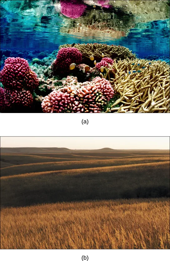
Current Species Diversity
Despite considerable effort, knowledge of the species that inhabit the planet is limited and always will be because of a continuing lack of financial resources and political willpower. A recent estimate suggests that the eukaryote species for which science has names, about 1.5 million species, account for less than 20 percent of the total number of eukaryote species present on the planet (8.7 million species, by one estimate). Estimates of numbers of prokaryotic species are largely guesses, but biologists agree that science has only begun to catalog their diversity. Even with what is known, there is no central repository of names or samples of the described species; therefore, there is no way to be sure that the 1.5 million descriptions is an accurate accounting. It is a best guess based on the opinions of experts in different taxonomic groups. Given that Earth is losing species at an accelerating pace, science is very much in the place it was with the Lake Victoria cichlids: knowing little about what is being lost. The table below presents recent estimates of biodiversity in different groups.
Estimates of the Numbers of Described and Predicted Species by Taxonomic Group
| Taxonomic Group | Mora et al. 2011 Described | Mora et al. 2011 Predicted | Chapman 2009 Described | Chapman 2009 Predicted | Groombridge & Jenkins 2002 Described | Groombridge & Jenkins 2002 Predicted |
|---|---|---|---|---|---|---|
| Animalia | 1,124,516 | 9,920,000 | 1,424,153 | 6,836,330 | 1,225,500 | 10,820,000 |
| Chromista | 17,892 | 34,900 | 25,044 | 200,500 | — | — |
| Fungi | 44,368 | 616,320 | 98,998 | 1,500,000 | 72,000 | 1,500,000 |
| Plantae | 224,244 | 314,600 | 310,129 | 390,800 | 270,000 | 320,000 |
| Protozoa | 16,236 | 72,800 | 28,871 | 1,000,000 | 80,000 | 600,000 |
| Prokaryotes | — | — | 10,307 | 1,000,000 | 10,175 | — |
| Total | 1,438,769 | 10,960,000 | 1,897,502 | 10,897,630 | 1,657,675 | 13,240,000 |
Sources: Mora Camilo et al., “How Many Species Are There on Earth and in the Ocean?” PLoS Biology (2011), doi:10.1371/journal.pbio.1001127; Arthur D. Chapman, Numbers of Living Species in Australia and the World, 2nd ed. (Canberra, AU: Australian Biological Resources Study, 2009), https://www.environment.gov.au/system/files/pages/2ee3f4a1-f130-465b-9c7a-79373680a067/files/nlsaw-2nd-complete.pdf; Brian Groombridge and Martin D. Jenkins, World Atlas of Biodiversity: Earth’s Living Resources in the 21st Century (Berkeley: University of California Press, 2002).
There are various initiatives to catalog described species in accessible ways, and the internet is facilitating that effort. Nevertheless, it has been pointed out that at the current rate of new species descriptions (which according to the State of Observed Species Report is 17,000 to 20,000 new species per year), it will take close to 500 years to finish describing life on this planet. (International Institute for Species Exploration (IISE), 2011 State of Observed Species (SOS). Tempe, AZ: IISE, 2011. Accessed May 20, 2012. http://www.esf.edu/species/.) Over time, the task becomes both increasingly difficult and increasingly easier as extinction removes species from the planet.
Naming and counting species may seem like an unimportant pursuit given the other needs of humanity, but determining biodiversity it is not simply an accounting of species. Describing a species is a complex process through which biologists determine an organism’s unique characteristics and whether or not that organism belongs to any other described species or genus. It allows biologists to find and recognize the species after the initial discovery, and allows them to follow up on questions about its biology. In addition, the unique characteristics of each species make it potentially valuable to humans or other species on which humans depend.
Patterns of Biodiversity
Biodiversity is not evenly distributed on Earth. Lake Victoria contained almost 500 species of cichlids alone, ignoring the other fish families present in the lake. All of these species were found only in Lake Victoria; therefore, the 500 species of cichlids were endemic. Endemic species are found in only one location. Endemics with highly restricted distributions are particularly vulnerable to extinction. Higher taxonomic levels, such as genera and families, can also be endemic. Lake Michigan contains about 79 species of fish, many of which are found in other lakes in North America. What accounts for the difference in fish diversity in these two lakes? Lake Victoria is an ancient tropical lake, while Lake Michigan is a recently formed temperate lake. Lake Michigan in its present form is only about 7,000 years old, while Lake Victoria in its present form is about 15,000 years old, although its basin is about 400,000 years in age. Biogeographers have suggested these two factors, latitude and age, are two of several hypotheses to explain biodiversity patterns on the planet.
Career Connection. Biogeographer
Biogeography is the study of the distribution of the world’s species—both in the past and in the present. The work of biogeographers is critical to understanding our physical environment, how the environment affects species, and how environmental changes impact the distribution of a species; it has also been critical to developing modern evolutionary theory. Biogeographers need to understand both biology and ecology. They also need to be well-versed in evolutionary studies, soil science, and climatology.
There are three main fields of study under the heading of biogeography: ecological biogeography, historical biogeography (called paleobiogeography), and conservation biogeography. Ecological biogeography studies the current factors affecting the distribution of plants and animals. Historical biogeography, as the name implies, studies the past distribution of species. Conservation biogeography, on the other hand, is focused on the protection and restoration of species based upon known historical and current ecological information. Each of these fields considers both zoogeography and phytogeography—the past and present distribution of animals and plants.
One of the oldest observed patterns in ecology is that species biodiversity in almost every taxonomic group increases as latitude declines. In other words, biodiversity increases closer to the equator, shown below.
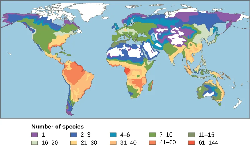
Extended description
The legend, titled “Number of species,” lists ten classes in two rows of five swatches each. Top row, left to right: purple for 1 species, blue for 2–3, teal for 4–6, green for 7–10, and olive green for 11–15. Bottom row, left to right: pale green for 16–20, tan for 21–30, light orange for 31–40, orange for 41–60, and red for 61–144. On the map, the reds and oranges (41–144 species) cover the Amazon basin of South America and parts of equatorial Africa; the coolest, palest colors (1–6 species) cover the northern edges of North America and Eurasia and the southern tip of South America; white patches mark areas with no data in this study.
It is not yet clear why biodiversity increases closer to the equator, but scientists have several hypotheses. One factor may be the greater age of the ecosystems in the tropics versus those in temperate regions; the temperate regions were largely devoid of life or were drastically reduced during the last glaciation. The idea is that greater age provides more time for speciation. Another possible explanation is the increased direct energy the tropics receive from the sun versus the decreased intensity of the solar energy that temperate and polar regions receive. Tropical ecosystem complexity may promote speciation by increasing the heterogeneity, or number of ecological niches, in the tropics relative to higher latitudes. The greater heterogeneity provides more opportunities for coevolution, specialization, and perhaps greater selection pressures leading to population differentiation. However, this hypothesis suffers from some circularity—ecosystems with more species encourage speciation, but how did they get more species to begin with?
The tropics have been perceived as being more stable than temperate regions, which have a pronounced climate and day-length seasonality. The tropics have their own forms of seasonality, such as rainfall, but they are generally assumed to be more stable environments and this stability might promote speciation into highly specialized niches.
Regardless of the mechanisms, it is certainly true that all levels of biodiversity are greatest in the tropics. Additionally, the rate of endemism is highest, and there are more biodiversity “hotspots.” However, this richness of diversity also means that knowledge of species is unfortunately very low, and there is a high potential for biodiversity loss.
Conservation of Biodiversity
In 1988, British environmentalist Norman Myers developed a conservation concept to identify areas rich in species and at significant risk for species loss: biodiversity hotspots. Biodiversity hotspots are geographical areas that contain high numbers of endemic species. The purpose of the concept was to identify important locations on the planet for conservation efforts, a kind of conservation triage. By protecting hotspots, governments are able to protect a larger number of species. The original criteria for a hotspot included the presence of 1500 or more endemic plant species and 70 percent of the area disturbed by human activity. There are now 34 biodiversity hotspots, shown below, containing large numbers of endemic species, which include half of Earth’s endemic plants.
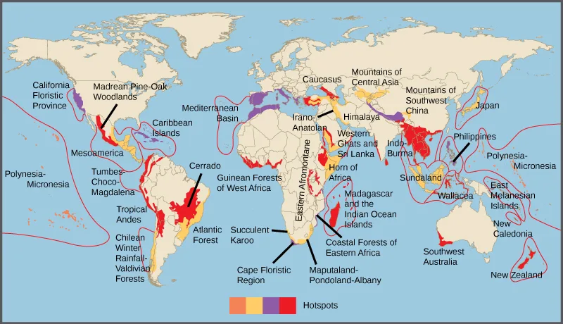
Extended description
Reading left to right across the map, the 34 labeled hotspots are: California Floristic Province, Madrean Pine-Oak Woodlands, Mesoamerica, Caribbean Islands, Tumbes-Choco-Magdalena, Tropical Andes, Cerrado, Atlantic Forest, and Chilean Winter Rainfall-Valdivian Forests in the Americas; Mediterranean Basin, Caucasus, Irano-Anatolian, Mountains of Central Asia, Himalaya, Western Ghats and Sri Lanka, Horn of Africa, Eastern Afromontane, Madagascar and the Indian Ocean Islands, Succulent Karoo, Cape Floristic Region, Maputaland-Pondoland-Albany, Guinean Forests of West Africa, and Coastal Forests of Eastern Africa across Europe, the Middle East, Asia, and Africa; and Mountains of Southwest China, Japan, Indo-Burma, Sundaland, Wallacea, Philippines, Southwest Australia, East Melanesian Islands, New Caledonia, and New Zealand across Asia and the Pacific, with Polynesia-Micronesia labeled at both the left and right edges of the map where the Pacific hotspot wraps around the projection.
Biodiversity Change through Geological Time
The number of species on the planet, or in any geographical area, is the result of an equilibrium of two evolutionary processes that are continuously ongoing: speciation and extinction. Both are natural “birth” and “death” processes of macroevolution. When speciation rates begin to outstrip extinction rates, the number of species will increase; likewise, the number of species will decrease when extinction rates begin to overtake speciation rates. Throughout Earth’s history, these two processes have fluctuated—sometimes leading to dramatic changes in the number of species on Earth as reflected in the fossil record, shown below.
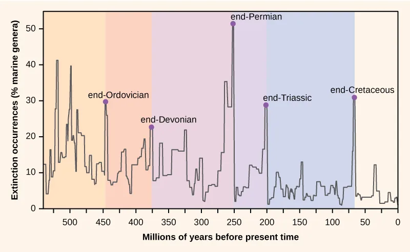
Extended description
The y-axis, “Extinction occurrences (% marine genera),” runs from 0 to just above 50 in increments of 10; the x-axis, “Millions of years before present time,” runs from about 550 down to 0, reading left to right toward the present. A jagged gray line traces extinction intensity across that span, with five purple dots marking the five mass extinctions, each labeled above its dot: end-Ordovician at about 450 million years ago and 30 percent; end-Devonian at about 375 million years ago and roughly 22 percent; end-Permian at about 250 million years ago and just over 50 percent, the tallest point on the graph; end-Triassic at about 200 million years ago and roughly 29 percent; and end-Cretaceous at about 66 million years ago and just over 30 percent. The plot area is shaded in background colors that change at three of those boundaries: tan from 550 to 450 million years ago, salmon from 450 to 375, lavender from 375 to 250, and pale blue from 250 to 66; a fifth, cream-colored band covers 66 million years ago to the present. The end-Triassic dot falls inside the pale blue band rather than at a color change.
Paleontologists have identified five strata in the fossil record that appear to show sudden and dramatic (between 25–55% of genera and greater than half of all extant species disappearing from the fossil record) losses in biodiversity. These are called mass extinctions. There are many lesser, yet still dramatic, extinction events, but the five mass extinctions have attracted the most research. An argument can be made that the five mass extinctions are only the five most extreme events in a continuous series of large extinction events throughout the Phanerozoic (since 542 million years ago). In most cases, the hypothesized causes are still controversial; however, the most recent mass extinction event seems clear.
The Five Mass Extinctions
The fossil record of the mass extinctions was the basis for defining periods of geological history, so they typically occur at the transition point between geological periods. The transition in fossils from one period to another reflects the dramatic loss of species and the gradual origin of new species. These transitions can be seen in the rock strata. The table below provides data on the five mass extinctions.
Mass Extinctions
| Geological Period | Mass Extinction Name | Time (millions of years ago) |
|---|---|---|
| Ordovician–Silurian | end-Ordovician O–S | 450–440 |
| Late Devonian | end-Devonian | 375–360 |
| Permian–Triassic | end-Permian | 251 |
| Triassic–Jurassic | end-Triassic | 205 |
| Cretaceous–Paleogene | end-Cretaceous K–Pg (K–T) | 65.5 |
The Ordovician-Silurian extinction event is the first recorded mass extinction and the second largest. During this period, about 85 percent of marine species (few species lived outside the oceans) became extinct. The main hypothesis for its cause is a period of glaciation and then warming. The extinction event actually consists of two extinction events separated by about 1 million years. The first event was caused by cooling, and the second event was due to the subsequent warming. The climate changes affected temperatures and sea levels. Some researchers have suggested that a gamma-ray burst, caused by a nearby supernova, was a possible cause of the Ordovician-Silurian extinction. The gamma-ray burst would have stripped away the Earth’s protective ozone layer, allowing intense ultraviolet radiation from the sun to reach the surface of the earth—and may account for climate changes observed at the time. The hypothesis is very speculative, and extraterrestrial influences on Earth’s history are an active line of research. Recovery of biodiversity after the mass extinction took from 5 to 20 million years, depending on the location.
The late Devonian extinction may have occurred over a relatively long period of time. It appears to have mostly affected marine species and not so much the plants or animals inhabiting terrestrial habitats. During this time 75 percent of all species became extinct. The causes of this extinction are poorly understood.
The end-Permian extinction was the largest in the history of life. Indeed, an argument could be made that Earth became nearly devoid of life during this extinction event. Estimates are that 96 percent of all marine species and 70 percent of all terrestrial species were lost. It was at this time, for example, that the trilobites, a group that survived the Ordovician–Silurian extinction, became extinct. The causes for this mass extinction are not clear, but the leading suspect is extended and widespread volcanic activity that led to a runaway global-warming event. The oceans became largely anoxic, suffocating marine life. Terrestrial tetrapod diversity took 30 million years to recover after the end-Permian extinction. The Permian extinction dramatically altered Earth’s biodiversity makeup and the course of evolution.
The causes of the Triassic–Jurassic extinction event are not clear, and researchers argue hypotheses including climate change, asteroid impact, and volcanic eruptions. The extinction event occurred just before the breakup of the supercontinent Pangaea, although recent scholarship suggests that the extinctions may have occurred more gradually throughout the Triassic. During this time 76 to 80 percent of all species became extinct.
The causes of the end-Cretaceous extinction event are the ones that are best understood. It was during this extinction event about 65 million years ago that the majority of the dinosaurs, the dominant vertebrate group for millions of years, disappeared from the planet (with the exception of a theropod clade that gave rise to birds). Overall, during this time period about 75 percent of all species became extinct.
The cause of this extinction is now understood to be the result of a cataclysmic impact of a large meteorite, or asteroid, off the coast of what is now the Yucatán Peninsula. This hypothesis, proposed first in 1980, was a radical explanation based on a sharp spike in the levels of iridium (which enters our atmosphere from meteors at a fairly constant rate but is otherwise absent on Earth’s surface) in the rock stratum that marks the boundary between the Cretaceous and Paleogene periods, shown below. This boundary marked the disappearance of the dinosaurs in fossils as well as many other taxa. The researchers who discovered the iridium spike interpreted it as a rapid influx of iridium from space to the atmosphere (in the form of a large asteroid) rather than a slowing in the deposition of sediments during that period. It was a radical explanation, but the report of an appropriately aged and sized impact crater in 1991 made the hypothesis more believable. Now an abundance of geological evidence supports the theory. Recovery times for biodiversity after the end-Cretaceous extinction are shorter, in geological time, than for the end-Permian extinction, on the order of 10 million years.
Another possibility, perhaps coincidental with the impact of the Yucatan asteroid, was extensive volcanism that began forming about 66 million years ago, about the same time as the Yucatan asteroid impact, at the end of the Cretaceous. The lava flows covered over 50 percent of what is now India. The release of volcanic gases, particularly sulfur dioxide, during the extensive eruptions contributed to climate change, which may have induced the mass extinction.
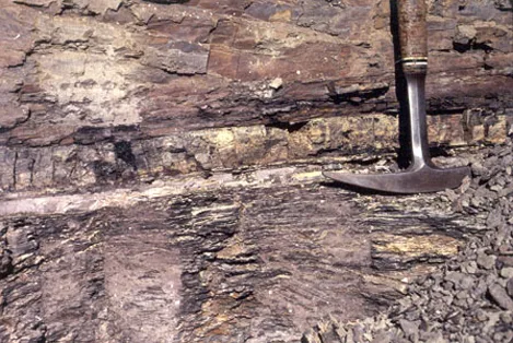
Scientists measured the relative abundance of fern spores above and below the K–Pg boundary in this rock sample. Which of the following statements most likely represents their findings?
Think about what a mass extinction event does to the diversity and abundance of a group’s fossils on the older side of a boundary compared with the younger side — the rock in this photo spans exactly that kind of transition.The Pleistocene Extinction
The Pleistocene Extinction is one of the lesser extinctions, and a recent one. It is well known that the North American, and to some degree Eurasian, megafauna—large vertebrate animals—disappeared toward the end of the last glaciation period. The extinction appears to have happened in a relatively restricted time period of 10,000–12,000 years ago. In North America, the losses were quite dramatic and included the woolly mammoths (with an extant population existing until about 4,000 years ago in isolation on Wrangel Island, Canada), mastodon, giant beavers, giant ground sloths, saber-toothed cats, and the North American camel, just to name a few. In the early 1900s, scientists first suggested the possibility that over-hunting caused the rapid extinction of these large animals. Research into this hypothesis continues today.
In general, the timing of the Pleistocene extinctions correlated with the arrival of paleo-humans, perhaps as long as 40,000 years ago, and not with climate-change events, which is the main competing hypothesis for these extinctions. The extinctions began in Australia about 40,000 to 50,000 years ago, just after the arrival of humans in the area: a marsupial lion, a giant one-ton wombat, and several giant kangaroo species disappeared. In North America, the extinctions of almost all of the large mammals occurred 10,000–12,000 years ago. All that are left are the smaller mammals such as bears, elk, moose, and cougars. Finally, on many remote oceanic islands, the extinctions of many species occurred coincidentally with human arrivals. Not all of the islands had large animals, but when there were large animals, they were often forced into extinction. Madagascar was colonized about 2,000 years ago and the large mammals that lived there became extinct. Eurasia and Africa do not show this pattern, but they also did not experience a recent arrival of hunter-gatherer humans. Rather, humans arrived in Eurasia hundreds of thousands of years ago. This topic remains an area of active research and hypothesizing. It seems clear that even if climate played a role, in most cases human hunting precipitated the extinctions.
Recent Extinctions
The sixth, or Holocene, mass extinction appears to have begun earlier than previously believed and is largely due to the disruptive activities of modern Homo sapiens. Since the beginning of the Holocene period, there are numerous recent extinctions of individual species that are recorded in human writings. Most of these are coincident with the expansion of the European colonies since the 1500s.
One of the earlier and popularly known examples is the dodo bird. The odd pigeon-like bird lived in the forests of Mauritius (an island in the Indian Ocean) and became extinct around 1662. The dodo was hunted for its meat by sailors and was easy prey because it approached people without fear (the dodo had not evolved with humans). Pigs, rats, and dogs brought to the island by European ships also killed dodo young and eggs.
Steller’s sea cow became extinct in 1768; it was related to the manatee and probably once lived along the northwest coast of North America. Steller’s sea cow was first discovered by Europeans in 1741 and was overhunted for meat and oil. The last sea cow was killed in 1768. That amounts to just 27 years between the sea cow’s first contact with Europeans and extinction of the species!
Since 1900, a variety of species have gone extinct, including the following:
- In 1914, the last living passenger pigeon died in a zoo in Cincinnati, Ohio. This species had once darkened the skies of North America during its migrations, but it was overhunted and suffered from habitat loss that resulted from the clearing of forests for farmland.
- The Carolina parakeet, once common in the eastern United States, died out in 1918. It suffered habitat loss and was hunted to prevent it from eating orchard fruit. (The parakeet ate orchard fruit because its native foods were destroyed to make way for farmland.)
- The Japanese sea lion, which inhabited a broad area around Japan and the coast of Korea, became extinct in the 1950s due to fishermen.
- The Caribbean monk seal was distributed throughout the Caribbean Sea but was driven to extinction via hunting by 1952.
These are only a few of the recorded extinctions in the past 500 years. The International Union for Conservation of Nature (IUCN) keeps a list of extinct and endangered species called the Red List. The list is not complete, but it describes 380 extinct species of vertebrates after 1500, 86 of which were driven extinct by overhunting or overfishing.
Estimates of Present-Time Extinction Rates
Estimates of extinction rates are hampered by the fact that most extinctions are probably happening without observation. The extinction of a bird or mammal is likely to be noticed by humans, especially if it has been hunted or used in some other way. But there are many organisms that are of less interest to humans (not necessarily of less value) and many that are undescribed.
The background extinction rate is estimated to be about one per million species per year (E/MSY). For example, assuming there are about ten million species in existence, the expectation is that ten species would become extinct each year.
One contemporary extinction rate estimate uses the extinctions in the written record since the year 1500. For birds alone this method yields an estimate of 26 E/MSY. However, this value may be an underestimate for three reasons. First, many species would not have been described until much later in the time period, so their loss would have gone unnoticed. Second, the number of recently extinct vertebrate species is increasing because extinct species now are being described from skeletal remains. And third, some species are probably already extinct even though conservationists are reluctant to name them as such. Taking these factors into account raises the estimated extinction rate closer to 100 E/MSY. The predicted rate by the end of the century is 1500 E/MSY.
A second approach to estimating present-time extinction rates is to correlate species loss with habitat loss by measuring forest-area loss and understanding species-area relationships. The species-area relationship is the rate at which new species are seen when the area surveyed is increased. Studies have shown that the number of species present increases as the size of the island increases. This phenomenon has also been shown to hold true in other island-like habitats as well, such as the mountain-top tepuis of Venezuela, which are surrounded by tropical forest. Turning this relationship around, if the habitat area is reduced, the number of species living there will also decline. Estimates of extinction rates based on habitat loss and species-area relationships have suggested that with about 90 percent habitat loss an expected 50 percent of species would become extinct. Species-area estimates have led to species extinction rate calculations of about 1000 E/MSY and higher. In general, actual observations do not show this amount of loss and suggestions have been made that there is a delay in extinction. Recent work has also called into question the applicability of the species-area relationship when estimating the loss of species. This work argues that the species-area relationship leads to an overestimate of extinction rates. A better relationship to use may be the endemics-area relationship. Using this method would bring estimates down to around 500 E/MSY in the coming century. Note that this value is still 500 times the background rate.
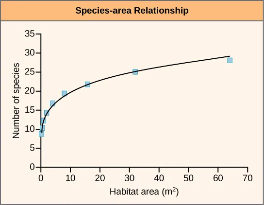
Extended description
The y-axis, “Number of species,” runs from 0 to 35 in increments of 5; the x-axis, “Habitat area (m²),” runs from 0 to 70 in increments of 10. Eight plotted data points rise steeply at first, from about 9 species at the smallest habitat area to about 17 species by 4 m², then more gradually to about 28 species at the largest plotted area, roughly 64 m², with a smooth curve fit through the points.
Summary
Biodiversity exists at multiple levels of organization and is measured in different ways depending on the scientific goals of those taking the measurements. These measurements include numbers of species, genetic diversity, chemical diversity, and ecosystem diversity. The number of described species is estimated to be 1.5 million with about 17,000 new species being described each year. Estimates for the total number of species on Earth vary but are on the order of 10 million. Biodiversity is negatively correlated with latitude for most taxa, meaning that biodiversity is higher in the tropics. The mechanism for this pattern is not known with certainty, but several plausible hypotheses have been advanced.
Five mass extinctions with losses of more than 50 percent of extant species are observable in the fossil record. Biodiversity recovery times after mass extinctions vary, but may be as long as 30 million years. Recent extinctions are recorded in written history and are the basis for one method of estimating contemporary extinction rates. The other method uses measures of habitat loss and species-area relationships. Estimates of contemporary extinction rates vary, but some rates are as high as 500 times the background rate, as determined from the fossil record, and are predicted to rise.
Key terms
- adaptive radiation — rapid branching through speciation of a phylogenetic tree into many closely related species
- biodiversity — variety of a biological system, typically conceived as the number of species, but also applying to genes, biochemistry, and ecosystems
- biodiversity hotspot — concept originated by Norman Myers to describe a geographical region with a large number of endemic species and a large percentage of degraded habitat
- chemical diversity — variety of metabolic compounds in an ecosystem
- ecosystem diversity — variety of ecosystems
- endemic species — species native to one place
- extinction — disappearance of a species from Earth; local extinction is the disappearance of a species from a region
- extinction rate — number of species becoming extinct over time, sometimes defined as extinctions per million species–years to make numbers manageable (E/MSY)
- genetic diversity — variety of genes in a species or other taxonomic group or ecosystem, the term can refer to allelic diversity or genome-wide diversity
- heterogeneity — number of ecological niches
- megafauna — large animals
- species-area relationship — relationship between area surveyed and number of species encountered; typically measured by incrementally increasing the area of a survey and determining the cumulative numbers of species
Practice
Define biodiversity in terms of species diversity and abundance
The number of currently described species on the planet is about ________.
The Current Species Diversity discussion gives one number for species science has already named and described, and a much larger number for its own rough guess at how many exist in total — pick the smaller, already-described figure.The variety of a biological system — typically thought of as the number of species, but also applied to genes, biochemistry, and ecosystems — is called ________.
Ecologists have separate words for genetic variety, chemical variety, and ecosystem variety; this is the umbrella word that covers all of them, defined in this section’s opening paragraph.A species found in only one location is called a(n) ________.
Lake Victoria’s now-vanished cichlids were an example of this kind of species — restricted to a single lake and nowhere else on Earth.Describe biodiversity as the equilibrium of naturally fluctuating rates of extinction and speciation
An adaptive radiation is________.
Both examples this section opens with, the Galápagos finches and the Lake Victoria cichlids, are famous not for anything to do with radioactivity, but for how many new species branched off from a common ancestor in a short span of time.With an extinction rate of 100 E/MSY and an estimated 10 million species, how many extinctions are expected to occur in a century?
E/MSY already scales the rate to a million species, so find how many million-species groups are in 10 million, multiply by the rate to get extinctions per year, then multiply by the number of years in a century.Describe the two methods used to calculate contemporary extinction rates.
Show model answer
Did your answer mention:
The relationship between the area surveyed and the number of species encountered, typically measured by increasing the surveyed area step by step and tracking the cumulative species count, is called the ________.
This is the second of the two methods for estimating present-time extinction rates described in this section — it works by shrinking or growing the size of a habitat and watching how many species come with it.Identify historical causes of high extinction rates in Earth’s history
A mass extinction is defined as ________.
The paragraph introducing the five mass extinctions gives a percentage range for lost genera and a separate, larger fraction for lost species overall — look for the species figure, not the genera range.Describe the evidence for the cause of the Cretaceous–Paleogene (K–Pg) mass extinction.
Show model answer
Did your answer mention:
Large vertebrate animals such as the woolly mammoth and giant ground sloth are collectively called ________.
This term names an entire group of animals by size alone — it comes up in this section’s discussion of the Pleistocene, when North America’s largest mammals disappeared.The complete disappearance of a species from Earth is called ________.
This section opens by contrasting the everyday, background rate of this process with five much larger spikes recorded in the fossil record.This section is adapted from Biology 2e, Section 47.1: The Biodiversity Crisis by Mary Ann Clark, Jung Choi, Matthew Douglas, and OpenStax, © OpenStax, licensed under CC BY-NC-SA 4.0. Access the original for free at openstax.org. Changes: figures re-encoded as WebP; four figures re-kinded from the manifest’s file-extension guess — Figure_47_01_02 (the amphibian species map), Figure_47_01_03 (the biodiversity hotspots map), Figure_B47_01_04-extinctions (the extinction-intensity graph), and Figure_47_01_06 (the species-area graph) from “photo” to “diagram,” and Figure_47_01_05 (the K–Pg boundary rock photo) from “diagram” to “photo”; Figure_47_01_01abf’s “photo” guess confirmed after inspection. Figure_47_01_05’s letter-spaced source alt (“K dash P g boundary”) rewritten in plain prose. Figure_47_01_03’s source alt, which named only a few of the 34 hotspots and misspelled “Australia” and “Caribbean” and printed “California cost” for “coast,” rewritten to describe the map generally, with the full list of 34 hotspots moved into a longdesc. Figure_B47_01_04-extinctions’s source alt (788 characters) shortened to fit the 600-character limit, with the peak readings moved into a longdesc that reads the drawn dots against the gridlines (about 22 percent for the late Devonian, 29 percent for the end-Triassic, and 66 million years ago for the end-Cretaceous, where the source alt says 25 percent, 30 percent, and roughly 70 million years ago — reported as a source defect). Longdescs added to Figure_47_01_02, Figure_47_01_03, Figure_B47_01_04-extinctions, and Figure_47_01_06, transcribing legend classes, the full list of labeled hotspots, the five labeled extinction peaks with their axis values, and the graph’s axis ranges and data trend, respectively. The Biogeographer Career Connection note rendered as a callout with its bold name and italicized title; the Link to Learning note rendered as a callout keeping its printed openstax.org/l/extinctions URL. Two source footnotes carrying full citations (Chapman 2009, whose citation also prints a URL, and the International Institute for Species Exploration’s 2011 State of Observed Species report) folded into parenthetical text, as elsewhere in the corpus; the Chapman citation’s URL kept as openstax.org/l/Aus_diversity; the IISE citation’s URL is printed without a hyperlink (see the end of this clause). Both source tables kept as Markdown tables in the body (no sortbins, since neither table’s columns name categories); the “Estimates of the Numbers of Described and Predicted Species by Taxonomic Group” table’s two-row header collapsed into one row per source column, and its three source citations moved to a sentence below it. In-text pointers to numbered figures and tables replaced with “shown above/below” or “the table above/below,” since Hugo does not number figures or tables. The body Visual Connection Question (fs-idp3595520) kept at the module’s own printed key, A — the module says nothing else about fern spores or the K–Pg fossil record beyond this item, so its own text cannot overturn the key; the end-matter exercise copy’s option C prints “boundary , and many” with a space before the comma (the in-body note copy already prints it correctly, “boundary, and many”), reported as a source defect, and the page uses the note copy’s correct spacing. The end-of-section Review Questions and Critical Thinking Questions adapted into the closing interactive Practice block, using every keyed exercise (fs-idm50545184, fs-idp36989440, fs-idp51516512, fs-idm88859952, fs-idm111141248, fs-idp2875584); rubric checkpoints added to both self-checks, decomposing each model answer (the source solution, lightly reformatted into complete sentences) into check-off clauses with no new claims. Five key-term recall items added from the glossary (biodiversity, endemic species, species-area relationship, megafauna, extinction), covering five of the section’s twelve glossary terms; the remaining seven (adaptive radiation, biodiversity hotspot, chemical diversity, ecosystem diversity, extinction rate, genetic diversity, heterogeneity) appear only in the prose and Key terms list. Objective groups assigned by subsection: “Types of Biodiversity,” “Current Species Diversity,” “Patterns of Biodiversity,” and “Conservation of Biodiversity” to the first objective; the “Biodiversity Change through Geological Time” introduction and “Estimates of Present-Time Extinction Rates” to the second (naturally fluctuating rates); “The Five Mass Extinctions,” “The Pleistocene Extinction,” and “Recent Extinctions” to the third (historical causes). No local items were needed; every Practice item traces to a keyed source exercise or the section’s own glossary; the State of Observed Species citation’s openstax.org redirect (/l/observed_species) is no longer a hyperlink — its destination, esf.edu/species, returned 404 on September 5, 2026, so the citation prints the URL as plain text (erratum 317).